
About a year ago, I joined a discussion on Reddit. A Reddit user requested to write several measurement points to the SQL database on the change of the value, with a timestamp. The value of the digital signals changed so that they were in the ON state for about 100 ms. He wrote that he could not use a SCADA system, which usually does not have a fast enough reading cycle.
Another user has written in several posts that the total data acquisition time (including writing to the SQL database) was not able to be less than 200 ms. My suggestion that they could use Raspberry Pi has received a critical response – the user considered it to be a slow and practically unusable device. And that in his experience, the transaction time (including all overhead) will not be stable below 100 ms. I quote:
"Of course, I can be wrong, but as I'm based on my experience the transaction time less than 100 ms might be not stable on standalone computers with Windows OS that are mostly used for such tasks."
Well, 100 ms seemed like a lot to me. In the past, when testing the performance of a PostgreSQL archive on a Raspberry Pi, we achieved hundreds of writes per second. This gives less than 10 ms for a single write. So - how's PostgreSQL really doing?
Therefore, I tried to configure a simple application in D2000, which would contain a Modbus TCP server with 100 measured points (in our terminology I/O tags) publishing values and a Modbus client that would read them once a second. Then I wanted to write these 100 values to the PostgreSQL archive database every second. The entire application server with the communication process, archive, and database would run on one computer. Can Raspberry handle it?
The hardware in use
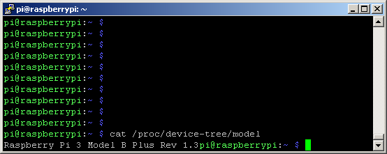
Let's go. I used a Raspberry Pi 3 model B Plus (not the latest model 4):
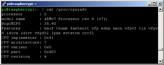
This model is equipped with 1GB of RAM and has a 4-core processor running at 1.3 GHz:
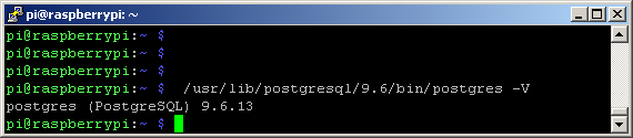
The installed PostgreSQL version was 9.6:
And the D2000 was version 12.0 Release 61.
Configuration
First, I created 2 lines of the "TCP-IP/TCP" type. The L.ModbusSrv line listened on port 502, at ALL address, which is a symbolic notation for listening on all network interfaces. The L.ModbusCliline was configured to connect to this port 502 on a loopback interface.
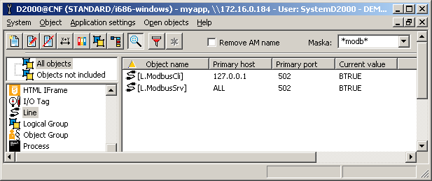
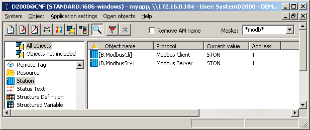
On the L.ModbusSrv line, I created the B.ModbusSrv station, configured the Modbus Server protocol, and entered address 1 on the Address tab. On the L.ModbusCli line, I created the B. ModbusCli station, configured the Modbus Client protocol, and entered again address 1 in the Address tab. I set the period of data reading to one second. Here is a view of both stations.
On the B.ModbusSrv station, I created 2 output I/O tags with addresses 3.0 and 3.1. This means that the Modbus Server will provide the values of these output I/O tags for request 3 (Read Holding Registers) from addresses 0 and 1 (see Modbus Server protocol documentation). Using CSV export, I exported the configuration of these I/O tags to a CSV file and in my favorite text editor PSPad, which supports block copying, replicated these I/O tags and created 100 I/O tags from them with addresses 3.0 to 3.99, as is shown in the following figure:
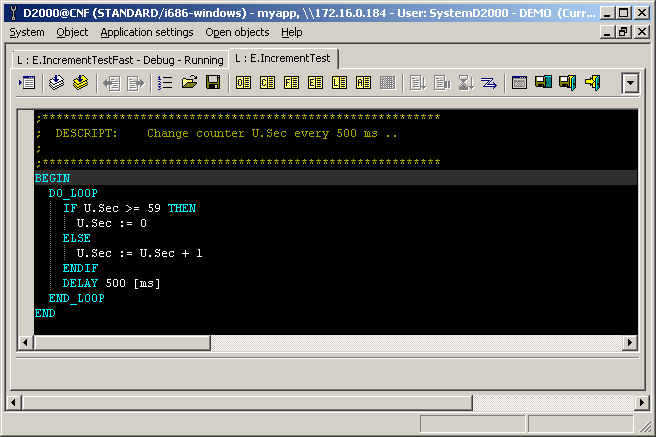
As a control object, I first used the system object Second (Sec), but later changed it to a user variable U.Sec, which I changed in the script about twice a second (to ensure, in accordance with the Shannon-Kotelnik theorem, fast enough changes that each client’s request received a different value). I changed the value from 0 to 59. Here is the corresponding script E.IncrementTest executed by the SELF.EVH process, which is also running on the Raspberry Pi:
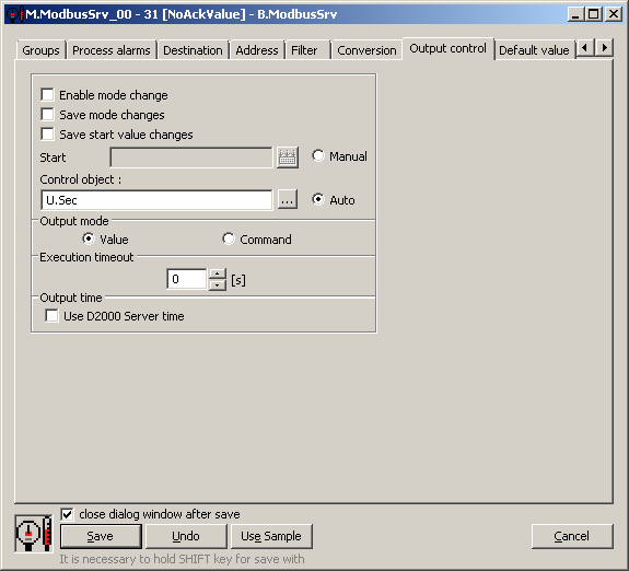
And here is the configuration of the Control object for one of the output I/O tags:
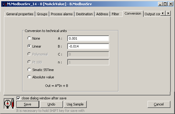
In order for each of the output I/O tags to publish a different value, I also configured the parameters of the linear conversion. For the N-th I/O tag (N = 0..99), I wanted the value 1000 * U.Sec + N.
That is, for example, I/O tag M.ModbusSrv_14 would publish a value of 14, 1014, 2014 .. etc, up to 59014.
However, since it is an output I/O tag and the conversion parameters are entered in the direction of input from the communication, it was necessary to perform an inverse conversion.
So if Y = 1000 * X + N, then X = Y/1000 - N/1000.
So the first coefficient (A) is 1/1000 = 0.001, the second coefficient (B) is -N / 1000 (different for each I/O tag). For the mentioned I/O tag M.ModbusSrv_14, the conversion will be as follows:
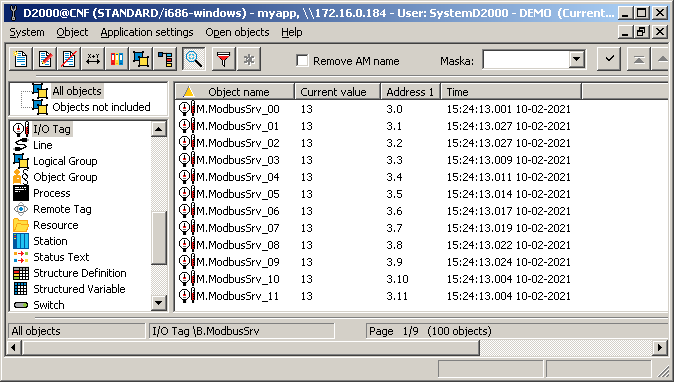
Similar to the I/O tags, I created 2 input I/O tags with addresses U3.0 and U3.1 on the B.ModbusCli station and replicated them to 100 I/O tags by exporting and importing. This time no conversion was required. The letter U in the address refers to the interpretation of the received value (2-byte Modbus register) as a positive number. The figure shows the I/O tags along with the current values and addresses:
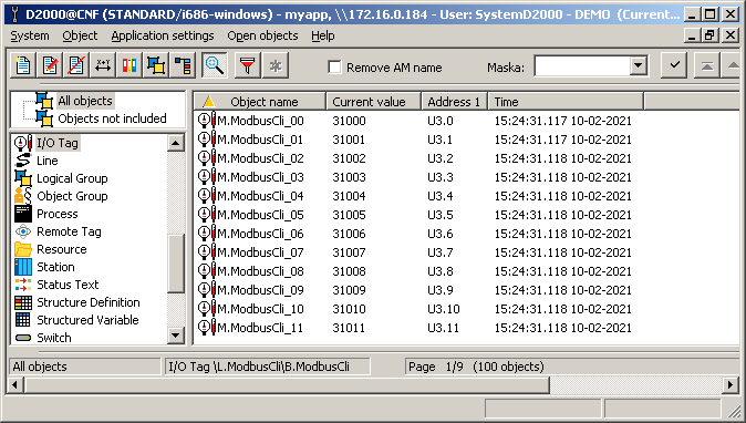
In each read cycle, a single Modbus request is sent to read registers 0 to 99, which is again answered by a single response.
The last step was the creation of two archive objects for archiving of the input I/O tags, and their replication using CSV export and import.
Testing
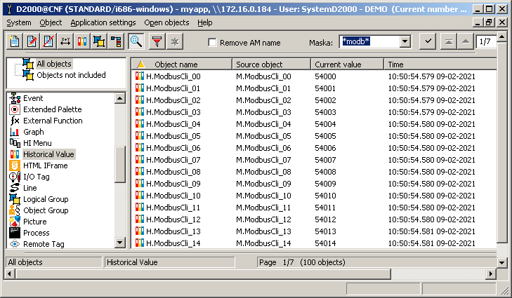
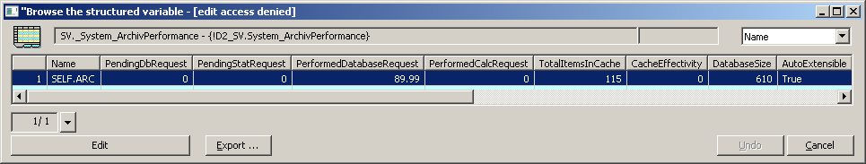
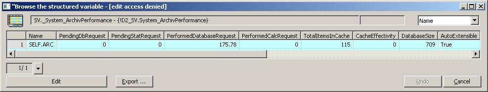
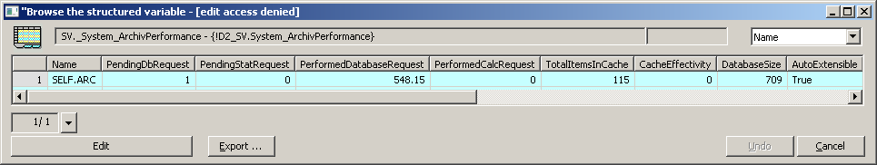
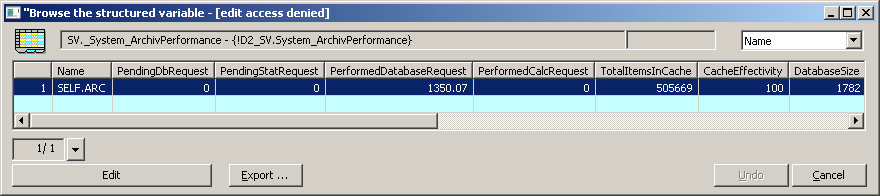
We also see the result of the whole effort in the system structure SV._System_ArchivPerformance. If we enter the name of the SELF.ARC archive process in the first column Name, the D2000 will start publishing statistics every 10 seconds. We see that PerformedDatabaseRequest is 100. So I archive 100 values every second (the number sometimes jumps higher due to other archive objects that exist in this application). At the same time, the value of PendingDbRequest is 0 or close to 0, so the SQL database catches up and no write requests accumulate in the archive queue.
How often is the database COMMIT performed? The default value is after 1000 written values resp. at least once every 60 seconds - these values can be changed, but I didn't do it. So we commit every 10 seconds.
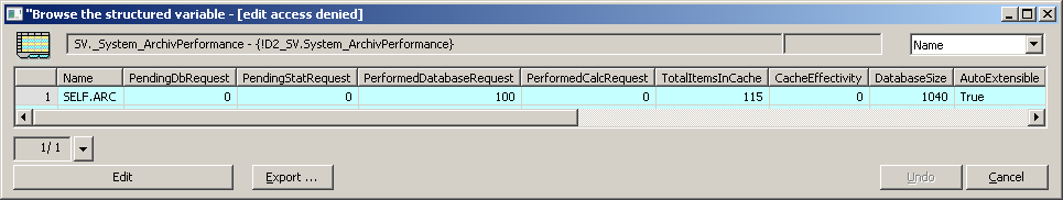
After approximately one day of running, the value of DatabaseSize, indicating the size of the archive database in MB, increased from 15 to 610. I made these tests at RPI with a 16 GB memory card, which had about 10 GB of free space. So it will last me a few more days.
The next morning, the database exceeded 1GB.
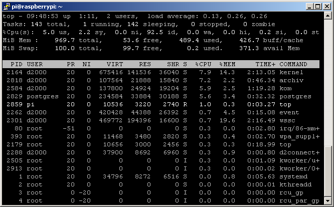
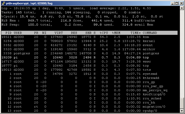
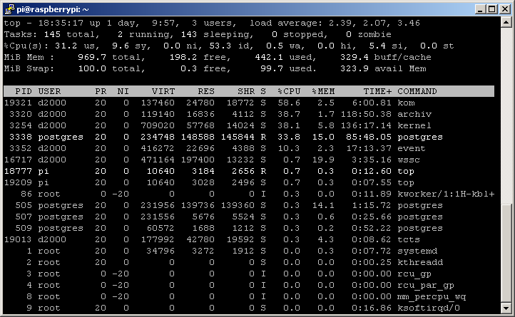
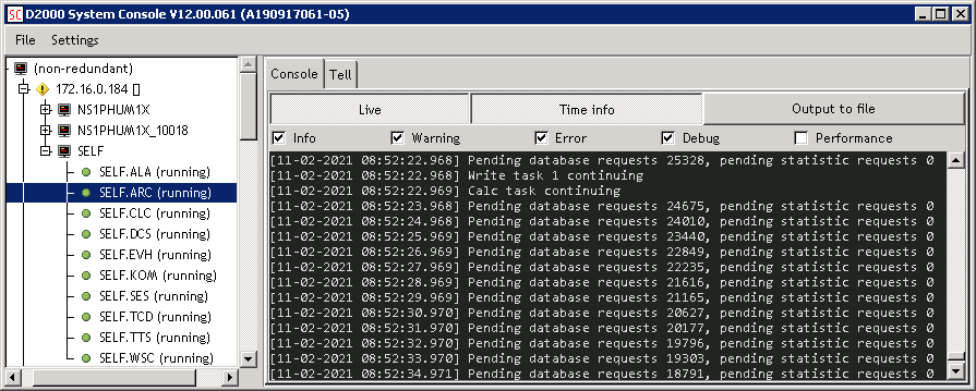
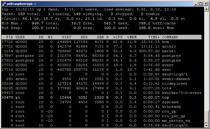
What is the load of RPI in such conditions? This is a screenshot shortly after configuration:
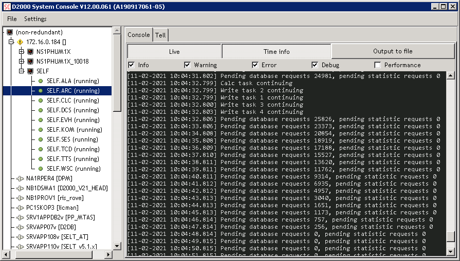
This is what the situation looks like after one day:
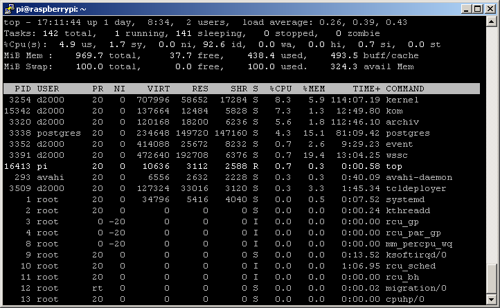
The numbers change, but above 1% of the CPU is consumed as expected by the kernel, kom, archive, and postgres processes.
Unintentional stress test
When I created the E.IncrementTest script to increment the U.Sec user variable, I – naturally - made a mistake and forgot to put a delay in the script (the line „DELAY 500 [ms]“). At the same time, I did not turn off the "Save start value" parameter when configuring U.Sec. The consequence of these two errors was that the script generated values of U.Sec as fast as it could, and the D2000 Server was saving them as startup values into the configuration database.
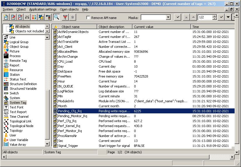
What is interesting from our point of view - how fast were these values stored? Again, the self-diagnostics of the D2000 system will help us. The Pending_Cfg_Rq system variable shows the number of configuration changes in the write queue (in our case, these are start values). The Perf_Cfg_Rq system variable shows how many writes have been made on average in the last 10 seconds. The CNF screenshot shows that more than 600 writes were made per second, while there are more than 6200 values in the write queue:
Of course, after realizing what I had done, I added a delay in the script and removed the saving of start values.
Archive database performance test
After less than a day of operation, I wanted to find out how quickly PostgreSQL can archive our values. The D2000 Archive has support for such stress tests - there is a FREEZE command that stops writing for a defined number of seconds (the first parameter of the command). It monitors the request queue every second and lists how many requests have accumulated in it. After the specified time, it unblocks the write task and continues monitoring (for a specified time - the second parameter of the command). The situation after running FREEZE 60 15 is shown in the picture:
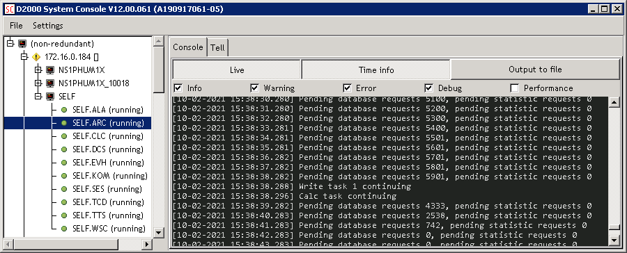
Over 5900 requests accumulated in the queue. In the first second of their processing, the number dropped to 4333, in the second to 2538, in the third to 742, and in the fourth to 0. This means that 5900 requests were processed in less than 4 seconds. In fact, there were 400 more of these requests as the communication continued to run, generating another 100 requests every second.
Frequent changes of a small number of I/O tags
After one day of trouble-free testing, I wanted to test a different configuration. What if there were only not 100 but only 10 I/O tags, however, their values would change often? How often can we change the value of a few I/O tags and how often can we read and archive them?
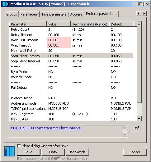
On the L.ModbusCli line, I configured another station B.ModbusCliFast with address 2. This time, I entered a zero delay in the time parameters (i.e. the “read as fast as possible” mode). I also adjusted the protocol parameters and reduced all waits to 1 ms. I created only 10 I/O tags on this station.
Of course, I also had to create a B.ModbusSrvFaststation with address 2 on the L.ModbusSrvline and the corresponding output I/O tags - but this time with the U.SecFast control object. I changed this in the script E.IncrementTestFast with a delay of 10 ms (of course, the actual delay may be greater and depends on the implementation).
I entered the station names B.ModbusCliFast and B.ModbusCli in the system structure SV._System_StationPerformance. This system structure allows you to get statistics on the number of changes at stations - which is exactly what I needed.
Note - I have not created archive objects for FastI/O tags yet.
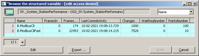
What do we see? Statistics for the last 10 seconds show that for the I/O tags belonging to the B.ModbusCli station, there are 1000 changes in 10 seconds as expected (corresponding to one change of each of the 100 points per second). As for the B.ModbusCliFaststation, there are about 7500 changes in 10 seconds, which corresponds to 75 changes of each of the 10 I/O tags every second. So the B.ModbusCliFast station manages to query the B.ModbusSrvFast station 75 times per second, process the responses, and publish the values. That's decent .. for a RPI.
What is a load of Raspberry Pi in such a mode? As expected, the load of the KOM process increased (almost 55% of the performance of one CPU core in the picture) - it originally had about 7%. The load of the D2000 Kernel has also increased (since all changes to objects must be processed).
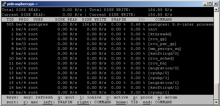
What is the load on the disks? The iotop utility usually shows a write of around 150 kB/sec.
The value of the Perf_Kernel_Rq system variable (the number of requests processed by the D2000 Server per second - again the average of the last 10 seconds) jumped to over 2200. Previously, it was around 400.

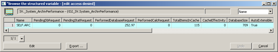
What happens when we archive these 10 fast I/O tags? We'll increase its load from 100 to 850 writes per second. I will do it gradually. After the creation of the first archive, the workload went from 100 to 175 writes:
Two archive objects - we are at 250, the archive is still doing fine:
We’ll add two more, we're at 400:

Two more archives, so we already have six. The load is about 550 writes per second.
Two more, the load goes to 700.

And the last two, we're at 850 archive writes per second. Importantly - PendingDbRequest is kept at 0, so the database manages to write.

How's the RPI? The workload of the archive increased from 5% to almost 40%. Postgres increased from 4% to 34%.
I left the system in this state for about 5 minutes, then I turned off these 10 demanding archives (especially so that I would not consume all the free space at night).
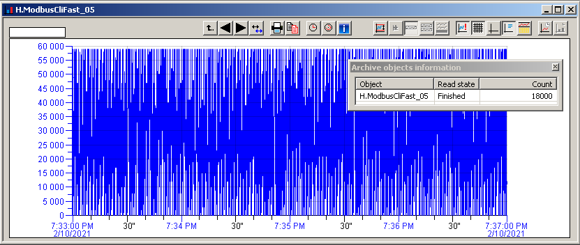
And now a look at archived data. This is what the 4 minutes graph looks, you can also see the information window that 18000 values have been read, which corresponds to 75 values per second.
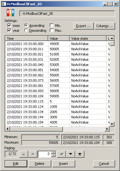
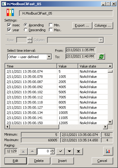
And here is a table with values. Timestamps (which are not supported by the Modbus protocol, so they are assigned by the D2000 KOM process when reading) are about 11-15 ms away. So responding to a signal change lasting 100 milliseconds shouldn't be a problem:
The next morning, I tried to turn on the archiving of fast archive objects again and then run the FREEZE 30 30 command (ie stop archiving for 30 seconds and then watch for another 30 seconds how the accumulated requests are processed). Approximately 850 requests are accumulated per second.
What do we see? In a second, the processing queue drops by about 400-600 requests. However, we must not forget that every second another 850 values from the communication are added, so the total flow to the archive was at the level of 1250-1450 requests per second.
There is one more thing to realize. The Raspberry Pi archive uses 1 write task by default. So there is still a performance reserve here. Let's try to configure 4 write tasks by setting a parameter
SELF.ARC.WriteThreadsCount = 4
in the application.properties file. Subsequently, an archive restart is required.
If we repeat the command FREEZE 30 30, you can see the result in the picture.
Approximately 25,000 accumulated requests were processed in 15 seconds, representing an average of 1,650 requests per second (plus another 850 of communications). This represents peak performance of up to 2500 writes per second. I give this number as a guide only, as it depends on other parameters of the application, archive, PostgreSQL database server, as well as the specific Raspberry Pi model used, including disk properties (for production deployment I would definitely prefer an external SSD disk over an SD card).
When I later thought about why we have "only" 75 changes of Fast I/O tags, I realized that there are two stations on a single Modbus line (slow B.ModbusCli and the new B.ModbusCliFast). However, I did not change the time parameters on the original station, which will cause a 100 ms waiting for a response after sending the request. So let’s make the last test - we turn off the B.ModbusCli station. Subsequently, the number of changes in the archive database reached almost 950 per second, which corresponds to 95 changes of each of the 10 fast I/O tags. Here we may already have a problem with not changing the values of the output I/O tags often enough. So let's try to reduce the delay in the E.IncrementTestFast script from 10 ms to 5 ms, so that the value of the output I/O tags changes 200 times per second. What happens?
We reached values around 1290 - 1390 per second. This means that RPI manages to execute 129-139 read requests per second. Of course, through the local interface, without network latency and similar effects. Further decreasing the delay in the script didn’t result in increase of input I/O tag changes.
This is what the values in the archive look like: the timestamps are 4-9 ms apart, at least every second change of value is captured.
In this mode, of course, the load of all processes is higher – the kom process went above 80%, the archive just below 80%, the kernel above 50% and the two write tasks of the PostgreSQL database together almost 70%. Yes, I decreased the number of write tasks from 4 down to 2, however without any significant effect.
Conclusion
I can only speculate why the Reddit user had such a negative view of the performance of the Raspberry Pi. It is possible that he tried data collection using a single-task application that simultaneously communicated, processed data and stored it in a database. The D2000 technology is modular, using multithreading and multitasking, asynchronous communication via priority queues, and thus effectively uses computer resources to maximize performance and prioritize time-critical activities.
In this blog, I wanted to show what possibilities and at the same time what limits the SCADA application deployed on Raspberry PI has. I think that the requirements for the collection and archiving of several digital signals, which change after about 100 milliseconds, is not a problem to achieve. If necessary, it would be possible e.g. to increase the priority of the D2000 KOM process - at the expense of archiving and kernel, database, and other processes that do not mind interruption for a few (tens of) milliseconds.
Some of our customers already use an industrial Raspberry clones (such as the Unipi or NPE X500) – as communication computers in production. Together with the KOM Archive functionality, which allows the D2000 KOM process to work offline (without a connection to the D2000 Server process - for example in case of network failure) and to save the values obtained from communication to a file (archive) for later transmission to the D2000 system, this is an effective and reliable communication solution.
When I talk about efficiency, I think of several parameters - performance, price, energy consumption. Speaking of reliability, when a Raspberry Pi is used as an application server, we can also offer redundant operation using two or more Raspberry Pis. Such a configuration significantly reduces the risk posed by an application server failure - whether it is a Raspberry Pi, an industrial computer, or a standard server. At the same time, the use of Raspberry Pi is effective in the scope of smaller applications (e.g. heat exchangers, waterworks, and other small industrial applications with a range of hundreds of tags).
At the same time, in this example, I wanted to point out the usefulness of D2000 system variables and other tools that allow to effectively determine the current performance of individual modules (communication, archiving, kernel) and then change their configuration parameters (such as the number of write tasks in the archive) to maximize the usage of computer resources. These features of the D2000 are even more useful in larger applications, where they help find sources of performance issues.
If you find this blog interesting and would like to try to compare the performance of the D2000 on your device (whether RPI or a different computer), you can easily do so. If you have RPI, download the RPI image and install it according to the instructions. Then download the XML export of all the objects I created for the needs of this blog.
Ing. Peter Humaj, www.ipesoft.com
